PyTorch cpu-only
pytorch
cpu
TensorFlow 2 cpu-only
tensorflow2
cpu
TensorFlow 1.15 cpu-only
tensorflow
cpu
PyTorch ROCm
pytorch
rocm
TensorFlow 2 ROCm
tensorflow2
rocm
PyTorch with AI Optimizer ROCm
opt-pytorch
rocm
TF2 with AI Optimizer ROCm
opt-tensorflow2
rocm
预构建Docker镜像支持列表
注意这里的Version一定要考虑其他依赖支不支持这个版本的Vitis AI,别上来直接latest。本文中拉取Pytorch的CPU版镜像(2.5.0)用于编译,运行
1 docker pull xilinx/vitis-ai-pytorch-cpu:2 .5 .0
但是,如果你想使用起来电脑上NVIDIA GPU的CUDA核,就要采取一些复杂的操作了,需要用Xilinx的Dockerfile构建自己的镜像。可以参见这里的官方文档 。(可能需要修改Dockerfile适应中国大陆网络)
进入Vitis AI根目录,修改一下docker_run.sh
找到docker_run_params , 删掉不存在的挂载参数
1
2
# -v /opt/ xilinx/dsa:/ opt/xilinx/ dsa \/opt/ xilinx/overlaybins:/ opt/xilinx/ overlaybins \
执行下面指令即可进入Vitis AI环境:
1 ./docker_run.sh xilinx/vitis-ai-pytorch-cpu:latest
Vitis AI
如果你没有修改过其他参数,那么Docker内的/workspace目录就是主机的Vitis-AI仓库根目录。
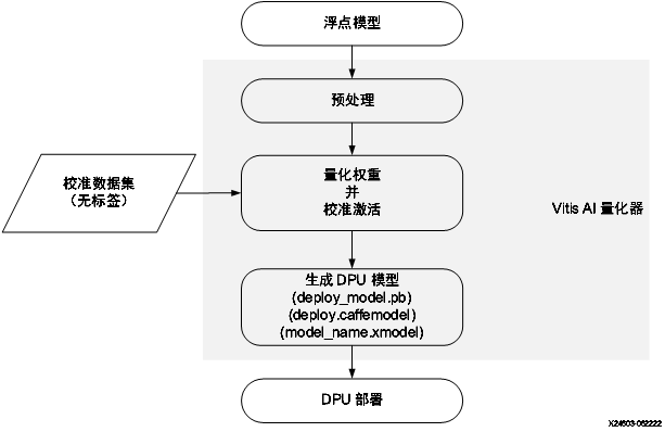
量化编译yolov5 该部分可参考UG1414 文档。大体流程如下:
首先克隆原始的Yolov5仓库,这里用的是ultralytics/yolov5 ,虽然ultralytics/ultralytics 也有yolov5,但因为增加了很多训练trick,导致源代码比较难修改,故采用前者。
克隆完后,安装所需要的依赖
1 pip install -i https://pypi.tuna.tsinghua.edu.cn/simple -r requirements.txt
修改模型 关于yolov5模型结构的介绍有很多,在此不一一介绍,一个比较显著的特点是,yolov5调整了激活函数,由ReLU改为了SiLU,但SiLU函数是不被DPU支持的,因此在训练之前,需要把激活函数换成ReLU或者LeakyReLU,找到yolov5仓库下的models文件夹,修改目标网络的yaml文件,加上以下文字:
训练&finetune 可以参考yolov5仓库下的说明文档,在其他机器上训练好或者finetune好导出成pytorch的pt文件即可。
量化 模型的量化可以参考Vitis-AI给出的demo , 可以看到量化分为calib和test两步,calib负责生成模型校准信息,test负责量化后xmodel的导出。
量化之前,需要对yolov5的代码再做一点修改,官方文档中指出量化模型应该仅包含forward方法,但在yolov5的源文件中(models/yolo.py ),可以看到以下代码
1
2
3
4
5
6
7
8
9
10
11
12
13
14
15
16
17
18
19
20
21
22
23
24
def forward (self, x ):for i in range (self .nl):self .m[i](x[i]) self .na, self .no, ny, nx).permute(0 , 1 , 3 , 4 , 2 ).contiguous()if not self .training: if self .dynamic or self .grid[i].shape[2 :4 ] != x[i].shape[2 :4 ]:self .grid[i], self .anchor_grid[i] = self ._make_grid(nx, ny, i)if isinstance (self , Segment): 2 , 2 , self .nc + 1 , self .no - self .nc - 5 ), 4 )2 + self .grid[i]) * self .stride[i] 2 ) ** 2 * self .anchor_grid[i] 4 )else : 2 , 2 , self .nc + 1 ), 4 )2 + self .grid[i]) * self .stride[i] 2 ) ** 2 * self .anchor_grid[i] 4 )self .na * nx * ny, self .no))return x if self .training else (torch.cat(z, 1 ),) if self .export else (torch.cat(z, 1 ), x)
这段代码在inference的时候,将预测的xy相对位置加上了grid坐标乘以stride来映射回原图,返回一个检测头的输出。但在这些步骤应该属于后处理的一部分,在量化的时候需要删掉,仅仅保留最纯正的网络输出x就可以了。
1
2
3
4
5
6
7
8
def forward(self , x ):for i in range(self .nl):x [i] = self .m[i](x [i]) # convx [i].shape # x (bs,255 ,20 ,20 ) to x (bs,3 ,20 ,20 ,85 )if self .grid[i].shape[2 :4 ] != x [i].shape[2 :4 ]:self .grid[i], self .anchor_grid[i] = self ._make_grid(nx, ny, i)return x
修改完后就可以开始写量化程序了,调用vai_q_pytorch的包可以很轻松的完成这一点,
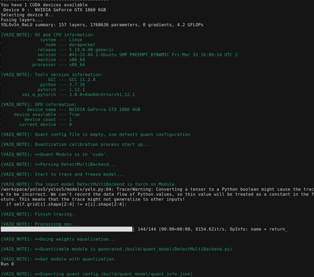
1
2
3
4
5
6
7
8
9
10
11
12
13
14
15
16
17
18
19
20
21
22
23
24
25
26
27
28
29
30
31
32
33
34
35
36
37
38
39
40
41
42
43
44
45
46
47
48
49
50
51
52
53
54
55
56
57
58
59
60
61
62
63
64
65
66
67
68
69
70
71
72
73
74
75
76
77
78
79
80
81
82
83
84
85
86
87
88
89
90
91
92
93
94
import osfrom pytorch_nndct.apis import torch_quantizer, dump_xmodelfrom common import *from models.common import DetectMultiBackendfrom models.yolo import Model'-----------------------------------------' '/dataset' '/float_model' '/quant_model' if available if (torch.cuda.device_count() > 0):print ('You have' ,torch.cuda.device_count(),'CUDA devices available' )for i in range(torch.cuda.device_count()):print (' Device' ,str(i),': ' ,torch.cuda.get_device_name(i))print ('Selecting device 0..' )'cuda:0' )else :print ('No CUDA devices available..selecting CPU' )'cpu' )"./v5n_ReLU_best.pt" , device =device)to merge BN with CONV for better quantization accuracyif in test modeif (quant_mode =='test'):output_dir =quant_model) '../../train/JPEGImages' ,transform =test_transform)batch_size =batchsize, shuffle =False )batch_size =1 if quant_mode == 'test' else 10, shuffle =False )export config if quant_mode == 'calib' :if quant_mode == 'test' :deploy_check =False , output_dir =quant_model)and parse the arguments'-d' , '--build_dir' , type =str, default ='build' , help ='Path to build folder. Default is build' )'-q' , '--quant_mode' , type =str, default ='calib' , choices=['calib' ,'test' ], help ='Quantization mode (calib or test). Default is calib' )'-b' , '--batchsize' , type =int, default =50, help ='Testing batchsize - must be an integer. Default is 100' )print ('\n' +DIVIDER)print ('PyTorch version : ' ,torch.__version__)print (sys.version)print (DIVIDER)print (' Command line options:' )print ('--build_dir : ' ,args.build_dir)print ('--quant_mode : ' ,args.quant_mode)print ('--batchsize : ' ,args.batchsize)print (DIVIDER)if __name__ == '__main__' :
量化的代码里面,调用了torch_quantizer来进行量化,量化后的模型一定要用数据集运行一遍(evaluate),可以是没有标签的纯图片,因为这些图片仅用于校准量化参数,不进行反向传播。
执行python文件来生成量化配置
1 python quantize.py -q calib
关注在此期间产生的Warning,比如未能识别的OP,这都是导致后面需要DPU分子图执行的原因。此时build/quant_model已经有生成的py了,需要接着运行test来生成xmodel
1 python quantize.py -q test -b 1
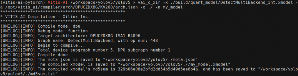
有了这个xmodel,我们需要用xilinx提供的compiler去把这个xmodel编译成DPU支持的,基于XIR的xmodel,运行如下指令:
1 vai_c_xir -x ./build/ quant_model/DetectMultiBackend_int.xmodel -a / opt/vitis_ai/ compiler/arch/ DPUCZDX8G/KV260/ arch.json -o ./ -n my_model
没有vai_c_xir?
keyboard_arrow_down
不知道是不是因为我安装的问题,我编译的GPU版本Vitis AI Docker找不到vai_c_xir这条指令,因此我使用GPU的Vitis AI量化生成xmodel以后,用CPU的预构建Docker来生成的最终xmodel
注意观察最终出来的DPU subgraph number是不是1,不是1的话请检查你的模型是不是有DPU不支持的OP,在遇到不支持的OP的时候,DPU会分为多个子图执行,由PS处理完后再发送给DPU,拖慢效率。生成的xmodel可以用netron查看网络输入输出结构。
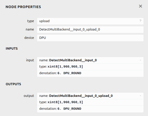
warning 仔细查看你的模型结构!一定要用netron查看网络输入输出结构,这点非常重要,因为输出以后的xmodel是一个量化模型,和原模型直接python跑不一样,在上板子部署的过程中需要将输入图片量化,并将量化输出转为浮点后再进行NMS等后处理流程。
我采用了自己训练的12分类的yolov5n模型,观察upload节点的输入如下图:
也就是说,输入图片是一个xint8的定点数,小数点在第6位,size是1*960*960*3。
有了生成的xmodel,模型部分的任务就结束了,接下来要进行部署
部署 部署前准备 首先我们需要一个DPU Design 的 Hardware,可以用Vivado手动Block Design搭一个,不过这会牵扯到很多麻烦的地址设置,我会另写文章单独讲,在这里我们简单用一下Xilinx搭建的标准DPU Hardware,在DPU-PYNQ仓库的boards文件夹 下就有。根据README 构建Design,需要安装xrt和Vitis。官方的脚本写的比较死板,只认2022.1的版本,可以编辑check_env.sh绕过检查
1
2
3
4
cd DPU-PYNQ/boardssource <vitis-install-path> /Vitis/2022.2 /settings64.sh source <xrt-install-path> /xilinx/xrt/setup.sh make BOARD=kv260_som
出现了Timing error?
keyboard_arrow_down
不知道为什么,笔者在构建的时候遇到了Timing问题,导致综合失败,我的解决方法是更换综合Strategy,修改/prj_config,[vivado]部分的最下面增加prop=run.impl_1.strategy=Performance_Explore,可以综合成功,不知道原来哪里出了问题。
脚本运行完后,会生成三个文件
dpu.bit
dpu.hwh
dpu.xclbin
再加上之前生成的
需要的文件都准备完成,接下来可以在pynq上进行部署。
安装DPU-PYNQ 配置好PYNQ环境后,需要单独安装DPU-PYNQ,这是一个包,提供了控制DPU的Python接口,位于下面的仓库中
可以直接通过pip安装
1
2
3
pip install pynq-dpu --no-build-isolation cd $PYNQ_JUPYTER_NOTEBOOKS pynq get-notebooks pynq-dpu -p .
运行后就可以使用pynq_dpu包了,并且会出现使用pynq_dpu的示例文件。
部署Yolov5 终于来到了激动人心的部署环节!为了让模型能运行起来,在ps需要做的是
部署DPU overlay,加载模型
前处理 + 量化输入
运行DPU推理
反量化输出 + 后处理
我们将一个个解决这些问题。
首先引入pynq-dpu包,这个包是针对pynq的封装,DpuOverlay是继承了Pynq Overlay的
1
2
3
from pynq_dpu import DpuOverlayoverlay = DpuOverlay("yolo5.bit" )"yolo5.xmodel" )
几个需要注意的点:
1、DpuOverlay的参数需要是bit文件,并且在同一路径 下应该有同名 的.xclbin和.hwh文件
2、编译生成的xmodel需要是上文vai_c_xir生成的xmodel,用test阶段生成的xmodel没用,且对于pynq-dpu来说,目前仅支持Vitis AI 2.5.0生成的xmodel。高版本编译生成的xmodel会导致notebook内核挂起。
然后定义输入输出的缓冲区:
1
2
3
4
5
6
7
8
9
10
11
12
13
14
15
16
17
18
dpu = overlay.runnerinputTensors = dpu.get_input_tensors()outputTensors = dpu.get_output_tensors()shapeIn = tuple(inputTensors[0 ].dims)shapeOut0 = (tuple(outputTensors[0 ].dims))shapeOut1 = (tuple(outputTensors[1 ].dims))shapeOut2 = (tuple(outputTensors[2 ].dims))outputSize0 = int(outputTensors[0 ].get_data_size() / shapeIn[0 ])outputSize1 = int(outputTensors[1 ].get_data_size() / shapeIn[0 ])outputSize2 = int(outputTensors[2 ].get_data_size() / shapeIn[0 ])input_data = [np.empty(shapeIn, dtype=np.int8, order="C" )]output_data = [np.empty(shapeOut0, dtype=np.int8, order="C" ), "C" ),"C" )]image = input_data[0 ]
在上面的代码中,outputTensors的大小应该和Netron中的一致。在本文中是1*120*120*36,1*60*60*36和1*30*30*36,对应yolov5-nano的三个检测头。
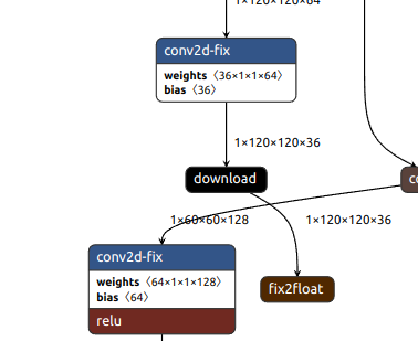
在netron中,DPU计算后输出的outputTensors表示为download 节点的数据类型,不是最后节点中的fix2float后的类型,这一步需要在cpu上自己做,如下图。
download节点
然后可以根据原来的全精度模型的推理代码写出DPU版本的推理代码,首先要对输入图像进行前处理。yolov5的输入是归一化后的像素值,且大小恒定,因此我们用原始代码中的letterbox进行大小裁剪后在对其进行归一化,然后对其进行int8量化。
1
2
3
4
5
6
7
im0 = cv2.imread('a.jpg')im = letterbox(im0, new_shape=(960 ,960 ), stride=32 )[0 ] # padded resizeim = im.transpose((2 , 0 , 1 )) # HWC to CHWim = np.ascontiguousarray(im) # contiguousim = np.transpose(im,(1 , 2 , 0 )).astype(np.float32) / 255 * (2 **6 ) # norm & quantif len(im.shape) == 3 :im = im[None] # expand for batch dim
在这段代码中,将图片进行padding后转置(opencv的通道和torch的通道位置不一样),并在最后一步/255归一化后*2^6,为什么是6次方呢?这时候就要用到图里的信息,上面贴过upload节点的数据,小数点是第六位的,因此是6次方,这里需要根据你的模型自己调整。
接下来将处理后的图像reshape成DPU input shape后送入DPU执行就可以了
1
2
3
image = im.reshape(shapeIn)is input_data
执行完毕后还需要对DPU结果进行反量化和整形,回顾一下在量化过程中的原始代码
1
2
3
4
5
6
7
8
9
10
11
12
13
14
15
16
17
18
19
20
21
22
23
24
def forward (self, x ):for i in range (self .nl):self .m[i](x[i]) self .na, self .no, ny, nx).permute(0 , 1 , 3 , 4 , 2 ).contiguous()if not self .training: if self .dynamic or self .grid[i].shape[2 :4 ] != x[i].shape[2 :4 ]:self .grid[i], self .anchor_grid[i] = self ._make_grid(nx, ny, i)if isinstance (self , Segment): 2 , 2 , self .nc + 1 , self .no - self .nc - 5 ), 4 )2 + self .grid[i]) * self .stride[i] 2 ) ** 2 * self .anchor_grid[i] 4 )else : 2 , 2 , self .nc + 1 ), 4 )2 + self .grid[i]) * self .stride[i] 2 ) ** 2 * self .anchor_grid[i] 4 )self .na * nx * ny, self .no))return x if self .training else (torch.cat(z, 1 ),) if self .export else (torch.cat(z, 1 ), x)
DPU的输出其实是模型输出,也就是x[i] = self.m[i]的这一部分输出,下面的reshape部分(x[i] = x[i].view(bs, self.na, self.no, ny, nx).permute(0, 1, 3, 4, 2))我们要自己补一下。
对于本模型的1*120*120*32的检测头,在yolov5后处理部分接受的数据是1*3*120*120*12的,因此需要先把32的维度提上来,进行拆分后再把12的部分转回去。
1
2
3
4
conv_out0 = np.transpose(output_data[0 ].astype(np.float32) / 4 , (0 , 3 , 1 , 2 )).view(1 , 3 , 12 , 120 , 120 ).transpose(0 , 1 , 3 , 4 , 2 )conv_out1 = np.transpose(output_data[1 ].astype(np.float32) / 8 , (0 , 3 , 1 , 2 )).view(1 , 3 , 12 , 60 , 60 ).transpose(0 , 1 , 3 , 4 , 2 )conv_out2 = np.transpose(output_data[2 ].astype(np.float32) / 4 , (0 , 3 , 1 , 2 )).view(1 , 3 , 12 , 30 , 30 ).transpose(0 , 1 , 3 , 4 , 2 )pred = [conv_out0, conv_out1, conv_out2]
在上面的代码中 从output_data拿出数据以后先进行了反量化,至于为什么/4,和量化的时候一样
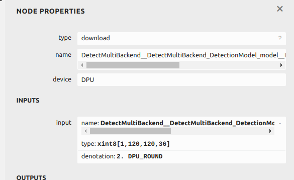
download节点信息
Download节点表明120大小的检测头输出的是小数点在第二位量化的结果,因此/4 即2^2。
接下来套用原来的后处理和nms即可,nms这里可能需要dump一下原模型的anchor信息,可以在原模型代码里直接访问模型参数拿到
1
2
3
4
5
6
model = DetectMultiBackend ('yolov5.pt' , device=device) print ("nc: " ,model.model.model[-1 ].nc) print ("anchors: " ,model.model.model[-1 ].anchors) print ("nl: " ,model.model.model[-1 ].nl) print ("na: " ,model.model.model[-1 ].na) print ("stride: " ,model.model.model[-1 ].stride)
后面就跟原始代码一样了,不过多赘述
结语 DPU最后这个模型的运行速度能达到50fps左右,已经很快了。但是主要卡在前处理上,如果模型过大的话resize会耗时,归一化的步骤也很耗时。不知道以后DPU会不会支持自己归一化,后面想搞一个把resize ip和DPU放在一起的设计,应该能加速很多。
感谢大家阅读。